aiR
aiR
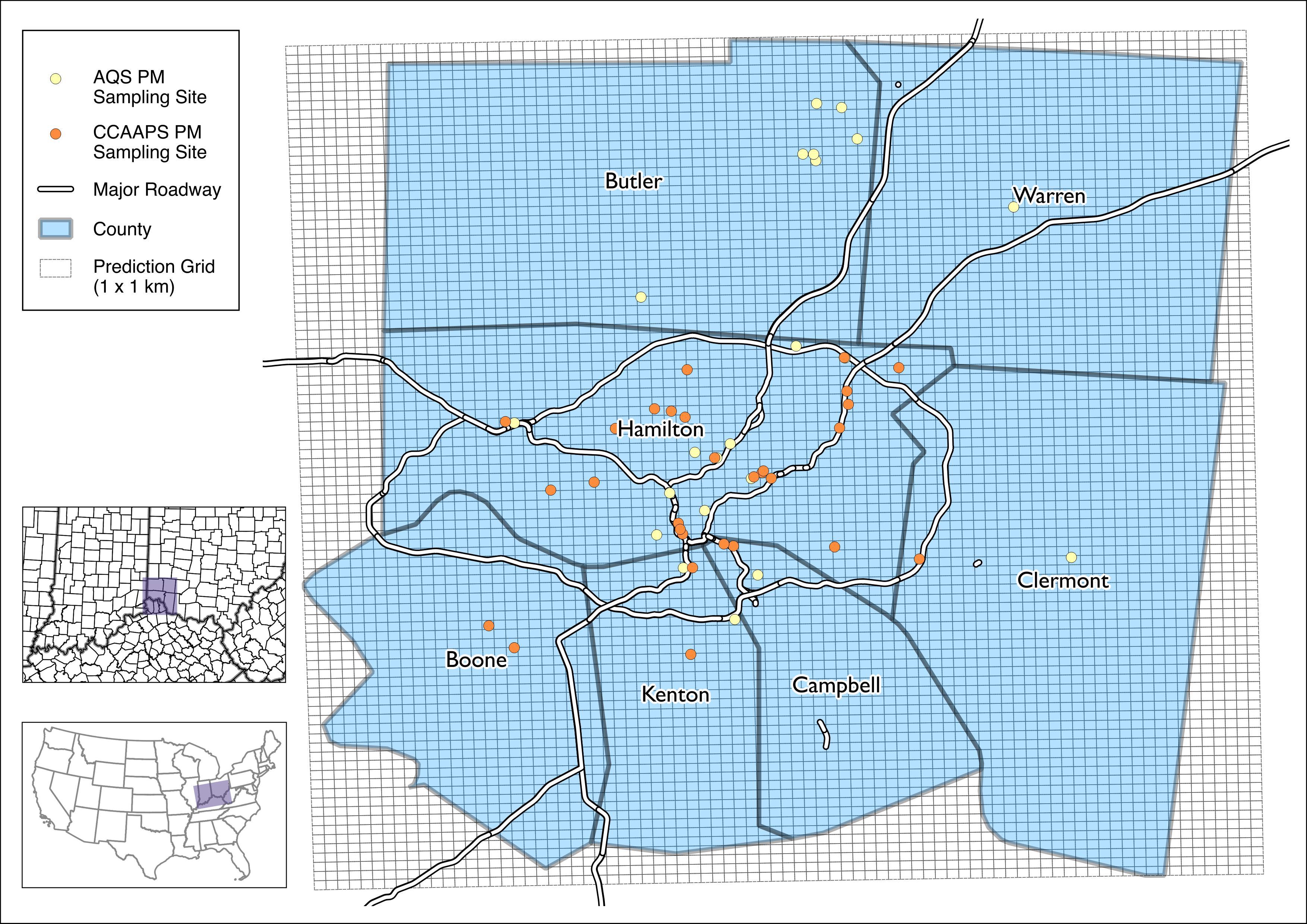
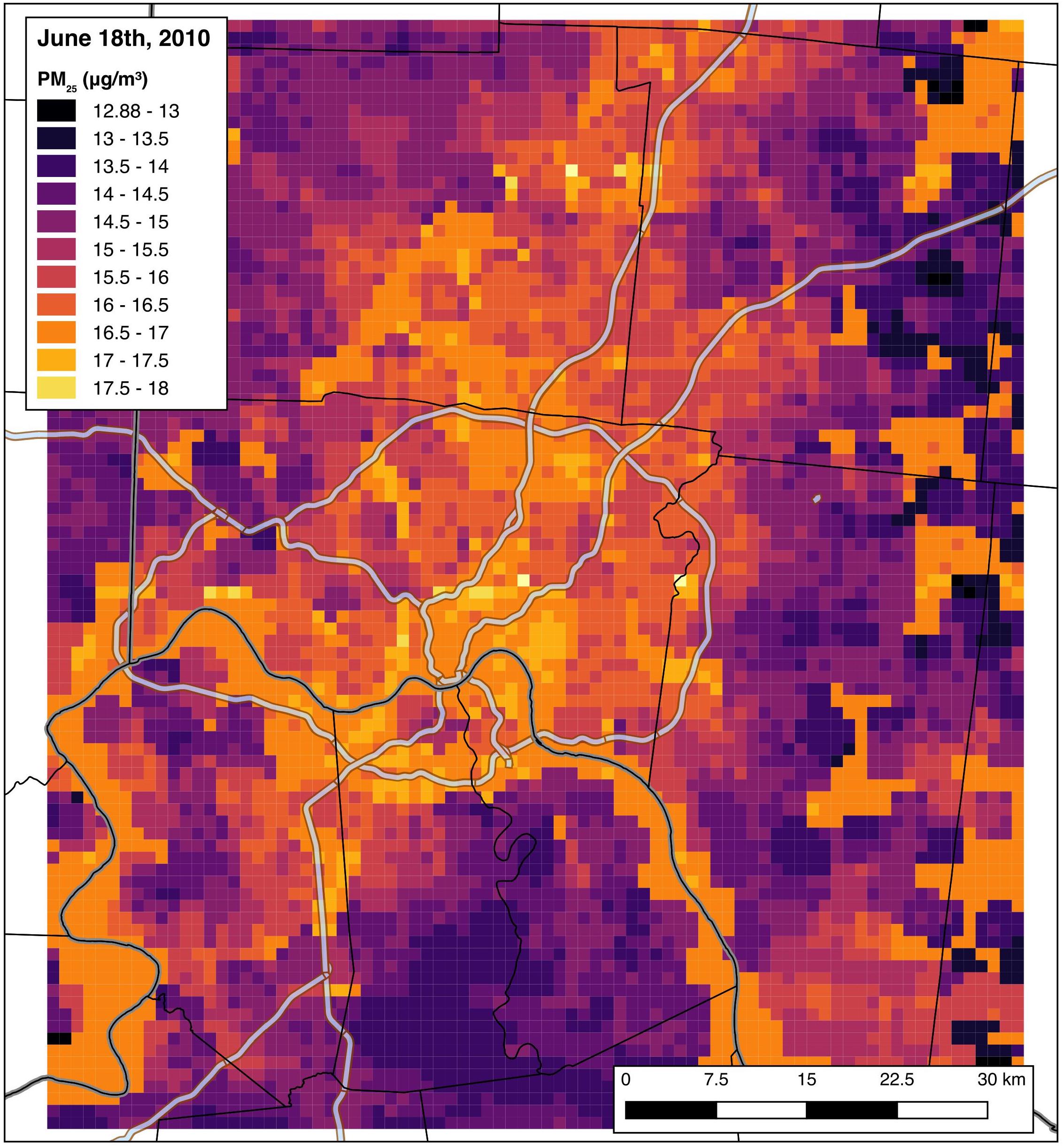
aiR is used to assess exposures to ambient particulate matter smaller than 2.5 micrometers (PM2.5) in the Cincinnati, Ohio area. The package creates predictions based on a spatiotemporal hybrid satellite/land use random forest model. Exposure predictions are available as daily averages at a 1 x 1 km grid resolution covering the “seven county” area (OH: Hamilton, Clermont, Warren, Butler; KY: Boone, Kenton, Campbell) from 2000 - 2015:
For example, below are the PM2.5 predictions for June 18th, 2010:
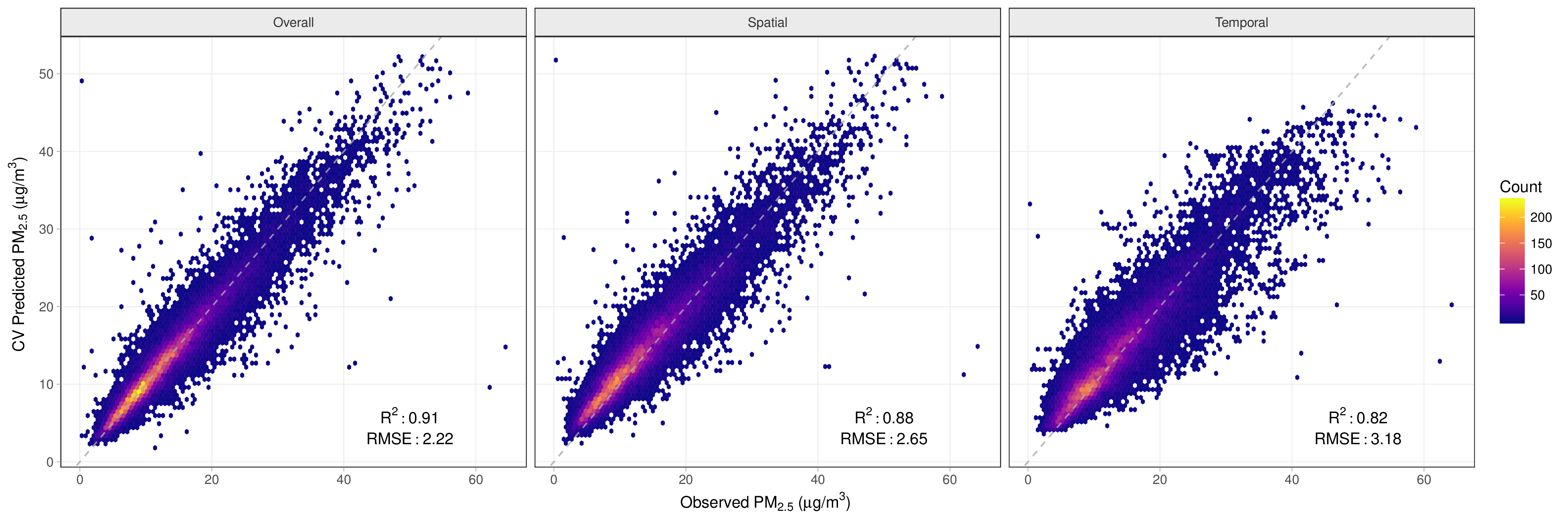
Cross validation of the model indicates that the PM2.5 predictions are excellent across the study domain, with a cross-validated median absolute error of 0.95 micrograms per cube meter and a cross-validated R2 of 0.91.
Reference
Please see our publication below for details on the data source, land use forest model, and cross validated accuracy. Please cite this manuscript if you use our package in a scientific publication:
Cole Brokamp, Roman Jandarov, Monir Hossain, Patrick Ryan. Predicting Daily Urban Fine Particulate Matter Concentrations Using Random Forest. Environmental Science & Technology. 52 (7). 4173-4179. 2018.
Installing
aiR is hosted on GitHub; install with:
remotes::install_github('cole-brokamp/aiR')
Example Usage
This example covers how to extract PM2.5 exposure estimates given latitude/longitude coordinates and dates.
Note that pm_grid and pm_data are both R objects that will be
available upon loading of the package. However, pm_data has to be
split into two smaller files (pm_data_early and pm_data_late) to be
under GitHub’s 100 MB filesize limit. This workaround requires binding
the two datasets into one upon package loading.
library(aiR)
library(tidyverse)
pm_data <- bind_rows(pm_data_early, pm_data_late)
Create a demonstration dataset of random coordinates and dates:
d <- tibble::tribble(
  ~id,         ~lon,        ~lat,
    809089L, -84.69127387, 39.24710734,
    813233L, -84.47798287, 39.12005904,
    814881L, -84.47123583,  39.2631309,
    799697L, -84.41741798, 39.18541228,
    799698L, -84.41395064, 39.18322447
  )

set.seed(12)

d <- d %>%
    mutate(date = seq.Date(as.Date('2015-01-01'), as.Date('2015-12-31'), by = 1) %>%
             base::sample(size=nrow(d)))
Convert this to a simple features object and transform to the Ohio South
projection. Reprojection is necessary because pm_grid is in the Ohio
South projection.
library(sf)
#> Linking to GEOS 3.6.1, GDAL 2.1.3, PROJ 4.9.3

d <- d %>%
  st_as_sf(coords = c('lon', 'lat'), crs=4326) %>%
    st_transform(3735)
To estimate the exposures, we will first overlay the locations with the
PM2.5 exposure grid to generate the pm_grid_id for each location.
( d <- st_join(d, pm_grid) )
#> Simple feature collection with 5 features and 3 fields
#> geometry type:  POINT
#> dimension:      XY
#> bbox:           xmin: 1347996 ymin: 414089 xmax: 1426020 ymax: 466143.5
#> epsg (SRID):    3735
#> proj4string:    +proj=lcc +lat_1=40.03333333333333 +lat_2=38.73333333333333 +lat_0=38 +lon_0=-82.5 +x_0=600000 +y_0=0 +ellps=GRS80 +towgs84=0,0,0,0,0,0,0 +units=us-ft +no_defs
#> # A tibble: 5 x 4
#>       id date       pm_grid_id                 geometry
#>    <int> <date>     <chr>      <POINT [US_survey_foot]>
#> 1 809089 2015-01-26 3016               (1347996 461745)
#> 2 813233 2015-10-25 4249               (1407370 414089)
#> 3 814881 2015-12-09 2954             (1410421 466143.5)
#> 4 799697 2015-04-08 3687             (1425054 437515.5)
#> 5 799698 2015-03-03 3688               (1426020 436698)
Then merge the “lookup grid” (pm_grid) into the dataset by using
pm_grid_id and date. Note that for the merge to work, the date
column must be named date and be of class Date and the pm_grid_id
column must exist.
( d <- left_join(d, pm_data, by = c('pm_grid_id', 'date')) )
#> Simple feature collection with 5 features and 4 fields
#> geometry type:  POINT
#> dimension:      XY
#> bbox:           xmin: 1347996 ymin: 414089 xmax: 1426020 ymax: 466143.5
#> epsg (SRID):    3735
#> proj4string:    +proj=lcc +lat_1=40.03333333333333 +lat_2=38.73333333333333 +lat_0=38 +lon_0=-82.5 +x_0=600000 +y_0=0 +ellps=GRS80 +towgs84=0,0,0,0,0,0,0 +units=us-ft +no_defs
#> # A tibble: 5 x 5
#>       id date       pm_grid_id pm_pred                 geometry
#>    <int> <date>     <chr>        <dbl> <POINT [US_survey_foot]>
#> 1 809089 2015-01-26 3016         18.4          (1347996 461745)
#> 2 813233 2015-10-25 4249          6.13         (1407370 414089)
#> 3 814881 2015-12-09 2954         14.9        (1410421 466143.5)
#> 4 799697 2015-04-08 3687          6.68       (1425054 437515.5)
#> 5 799698 2015-03-03 3688         13.9          (1426020 436698)
Adding Weather Data
Several NARR weather variables are available as daily means for the
entire study area in the narr_data R object. View the help
(?narr_data) to see more details about the individual variables.
To merge in humidity and temperature, we will subset narr_data to
those variables and join to our dataset:
( d <- left_join(d, narr_data %>% select(date, air.2m, rhum.2m), by = 'date') )
#> Simple feature collection with 5 features and 6 fields
#> geometry type:  POINT
#> dimension:      XY
#> bbox:           xmin: 1347996 ymin: 414089 xmax: 1426020 ymax: 466143.5
#> epsg (SRID):    3735
#> proj4string:    +proj=lcc +lat_1=40.03333333333333 +lat_2=38.73333333333333 +lat_0=38 +lon_0=-82.5 +x_0=600000 +y_0=0 +ellps=GRS80 +towgs84=0,0,0,0,0,0,0 +units=us-ft +no_defs
#> # A tibble: 5 x 7
#>       id date       pm_grid_id pm_pred air.2m rhum.2m
#>    <int> <date>     <chr>        <dbl>  <dbl>   <dbl>
#> 1 809089 2015-01-26 3016         18.4    273.    84.2
#> 2 813233 2015-10-25 4249          6.13   290.    72.2
#> 3 814881 2015-12-09 2954         14.9    280.    86.9
#> 4 799697 2015-04-08 3687          6.68   292.    84.6
#> 5 799698 2015-03-03 3688         13.9    272.    87.9
#> # … with 1 more variable: geometry <POINT [US_survey_foot]>